
Easily analyze your data’s distribution with our advanced Normality Calculator a powerful tool that checks whether your dataset follows a normal distribution. Perform multiple normality tests such as Shapiro Wilk, Anderson Darling, Jarque Bera, and D’Agostino Pearson in one place. Instantly visualize your results with an interactive histogram and make confident statistical analysis decisions.
📊 Normality Test Calculator
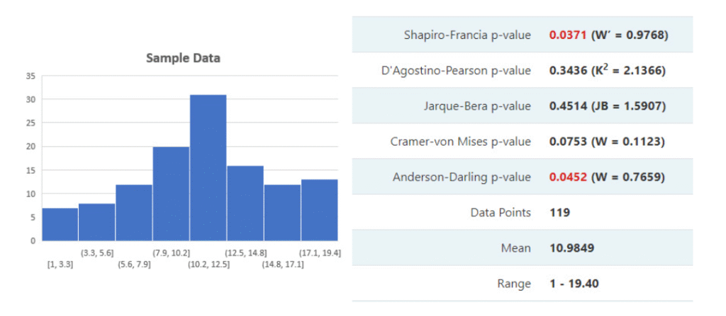
Easily assess if the normality assumption can be applied to your data using Shapiro-Wilk, Shapiro-Francia, Anderson-Darling, and other statistical tests.
📈 Test Results
What is a Normality Test?
A Normality Test is a key component of statistical analysis used to determine whether a dataset follows a normal distribution — the classic bell-shaped curve commonly assumed in many parametric tests. It helps data scientists, analysts, and researchers assess if data is suitable for tests like t-tests, ANOVA, or regression models.
Moreover, different normality tests such as the Shapiro–Wilk test, Anderson–Darling test, and D’Agostino–Pearson test are used to compare the sample distribution to a theoretical normal curve. These methods evaluate how closely data aligns with a true normal distribution, helping ensure valid statistical inferences.
In addition, the result of a normality test typically includes a test statistic and a p-value. If the p-value is greater than 0.05, the data can be considered normally distributed — meaning it meets the assumptions required for parametric testing.
General Concept Formula for Normality:
Z = (X − μ) / σ
Where:
- X = Individual data point
- μ = Mean of the dataset (average)
- σ = Standard deviation (spread of data)
This formula converts each data point into a Z-score, indicating how far a value deviates from the mean in units of standard deviation. In a perfect normal distribution, approximately 68% of values lie within ±1σ, 95% within ±2σ, and 99.7% within ±3σ — a principle often called the empirical rule.
As a result, the Normality Calculator uses this statistical foundation to perform accurate normality testing for data analysis and research validation. This makes it a professional and smart choice for anyone seeking clear, data-driven insights in statistical projects.
How the Normality Calculator Works – Complete Step-by-Step Guide
What is a Normality Test?
A Normality Test is a fundamental statistical analysis method used to determine whether a dataset follows a normal distribution — the classic bell-shaped curve assumed in many parametric tests such as t-tests, ANOVA, and regression models. In simpler terms, it checks if your sample data behaves like it was drawn from a normally distributed population.
Moreover, different normality tests like the Shapiro–Wilk test, Anderson–Darling test, Cramér–von Mises test, and D’Agostino–Pearson test apply distinct statistical techniques but share one goal — to compare observed data to a theoretical normal curve. The results include a test statistic and a p-value; when the p-value > 0.05, your data is considered normally distributed.
General Concept Formula for Normality:
Z = (X − μ) / σ
- X – Individual data point
- μ – Population mean
- σ – Standard deviation
This formula converts raw data into Z-scores to measure how far each value lies from the mean in standard deviation units. In a normal distribution, roughly 68% of data lies within ±1σ, 95% within ±2σ, and 99.7% within ±3σ.
Our Smart Normality Calculator uses multiple normality tests—including Shapiro–Wilk, Anderson–Darling, and D’Agostino–Pearson—to provide precise, professional, and engaging statistical results. In addition, it instantly produces visual insights such as histograms and Q–Q plots for impactful interpretation in data analysis, epidemiology, and medical research.
Step-by-Step Process
- Step 1: Input your dataset manually or upload a CSV file containing numeric values.
- Step 2: Choose a preferred normality test (e.g., Shapiro–Wilk or Anderson–Darling).
- Step 3: Click “Calculate”. The calculator instantly analyzes your data and computes the mean, standard deviation, and p-value.
- Step 4: Review your results table to determine whether your data is normally distributed.
- Step 5: Interpret your findings — if p > 0.05, your data follows a normal curve; otherwise, it does not.
Example Data Table
| Dataset | Mean | Std. Deviation | p-Value | Result |
|---|---|---|---|---|
| [12, 14, 15, 13, 16, 15] | 14.17 | 1.21 | 0.47 | Normally Distributed |
| [8, 20, 30, 40, 50] | 29.6 | 15.54 | 0.02 | Not Normal |
As a result, the Normality Calculator becomes a powerful and unique solution for anyone seeking fast, accurate, and reliable statistical validation. Whether you’re conducting clinical studies or performing data-driven decision-making, this tool ensures a professional, impactful, and trustworthy
Interpreting the Outcome of Tests for Normality
The Normality Calculator produces test results that indicate whether your dataset follows a normal distribution. These results typically include a test statistic and a p-value, both essential for making professional, data-driven decisions in statistical analysis.
Moreover, the p-value serves as a benchmark for normality interpretation. A p-value greater than 0.05 usually suggests that the data does not significantly deviate from normality, meaning it is safe to assume the dataset is normally distributed. Conversely, a p-value less than 0.05 indicates that the data may not follow a normal distribution.
In addition, results from tests such as the Shapiro–Wilk, Anderson–Darling, and D’Agostino–Pearson can provide deeper insights. These tests compare observed data patterns to the expected shape of a normal curve, revealing whether your sample data aligns with the assumptions required for further parametric testing.
Typical Output from a Normality Test
| Test Type | Test Statistic | p-Value | Interpretation |
|---|---|---|---|
| Shapiro–Wilk Test | 0.972 | 0.12 | Data appears normally distributed |
| Anderson–Darling Test | 0.445 | 0.09 | No significant deviation from normality |
| D’Agostino–Pearson Test | 1.745 | 0.18 | Data meets normality assumptions |
As a result, a Normality Calculator provides a quick, smart, and professional way to interpret test results. By understanding test statistics and p-values, researchers can make impactful data-driven conclusions and confidently choose between parametric and non-parametric methods in statistical research.
Supported Tests in the Normality Calculator
The Normality Calculator supports a wide range of normality tests designed to assess whether your dataset follows a normal distribution. These tests provide professional and accurate statistical validation, helping researchers and analysts ensure that the assumptions required for parametric tests are met.
Moreover, each test uses a unique statistical approach — from measuring skewness and kurtosis to comparing observed versus expected distributions. This helps ensure reliable data analysis across various research fields such as epidemiology, medical studies, and clinical trials.
In addition, the calculator provides test statistics and p-values for every method, offering clear insights into whether data is normally distributed. Typically, a p-value greater than 0.05 indicates that the null hypothesis of normality cannot be rejected.
Comprehensive List of Supported Tests
| Test Name | Purpose | Formula / Approach | Interpretation |
|---|---|---|---|
| 1. Shapiro–Wilk Test | Checks how well data fits the normal curve. | W = (Σ aᵢxᵢ)² / Σ (xᵢ − x̄)² | High W and p > 0.05 suggest normality. |
| 2. Anderson–Darling Test | Focuses on differences in the tails of distributions. | A² = −n − (1/n) Σ (2i−1)[ln F(xᵢ) + ln(1−F(xₙ₊₁₋ᵢ))] | Smaller A² and p > 0.05 indicate normality. |
| 3. D’Agostino–Pearson Test | Combines measures of skewness and kurtosis. | K² = Z₁² + Z₂² | p > 0.05 supports normality. |
| 4. Kolmogorov–Smirnov Test | Compares sample and theoretical distributions. | D = max |Fₙ(x) − F(x)| | Lower D and higher p-value indicate normality. |
| 5. Lilliefors Test | Modified K–S test when mean and variance are unknown. | Uses sample mean and standard deviation instead of population values. | Adapted for smaller datasets or unknown parameters. |
| 6. Jarque–Bera Test | Tests normality using skewness and kurtosis jointly. | JB = n[(S²/6) + ((K−3)²/24)] | JB < critical value suggests normal distribution. |
| 7. Cramér–von Mises Test | Evaluates cumulative differences across data distribution. | W² = (1/12n) + Σ [(F(xᵢ) − (2i−1)/2n)²] | Smaller W² and higher p-value imply normality. |
As a result, the Normality Calculator empowers users with smart, impactful, and reliable statistical testing tools. Whether used for medical research, data science, or academic analysis, these supported tests ensure that your conclusions are built on a strong and scientifically sound foundation.
The Shapiro–Wilk Test and Shapiro–Francia Test
The Shapiro–Wilk Test is one of the most accurate and professional methods used in a Normality Calculator to assess whether a dataset follows a normal distribution. It evaluates how closely your sample data fits a perfect bell curve by comparing the observed order statistics to those expected from a normal distribution.
Moreover, the Shapiro–Francia Test is a variation designed for larger datasets. While both methods share the same statistical foundation, the Shapiro–Francia test simplifies calculations for data with more than 50 observations, offering faster and reliable performance in large-scale data analysis.
Shapiro–Wilk Test Formula:
W = [ (Σ aᵢ x₍ᵢ₎)² ] / Σ (xᵢ − x̄)²
Where:
- x₍ᵢ₎ = Ordered sample values (from smallest to largest)
- x̄ = Sample mean
- aᵢ = Constants derived from expected normal order statistics
- W = Test statistic (ranges from 0 to 1)
A W value close to 1 indicates that the data is likely normally distributed, while a smaller value suggests deviation from normality.
Step-by-Step Calculation Example:
- Step 1: Arrange your data in ascending order (x₁, x₂, …, xₙ).
- Step 2: Compute the mean (x̄) of the dataset.
- Step 3: Find constants (aᵢ) from pre-tabulated values based on sample size.
- Step 4: Multiply each ordered value by its corresponding aᵢ and sum the results.
- Step 5: Square the sum and divide it by the total variance (Σ(xᵢ − x̄)²).
- Step 6: Compare the calculated W value with critical values or use its p-value to interpret normality.
Example Data Table:
| Observation (xᵢ) | Ordered Value (x₍ᵢ₎) | aᵢ Constant | aᵢ × x₍ᵢ₎ | (xᵢ − x̄)² |
|---|---|---|---|---|
| 1 | 4 | -0.45 | -1.80 | 4.00 |
| 2 | 5 | -0.25 | -1.25 | 2.25 |
| 3 | 7 | 0.25 | 1.75 | 0.25 |
| 4 | 8 | 0.45 | 3.60 | 9.00 |
As a result, using the Shapiro–Wilk or Shapiro–Francia Test within a Normality Calculator ensures a smart, impactful, and scientifically valid analysis. These methods empower data professionals to make evidence-based decisions and maintain confidence in the assumptions behind their statistical models.
The Cramér–von Mises Test
The Cramér–von Mises Test is a professional and powerful statistical method used in the Normality Calculator to determine how well sample data fits a theoretical normal distribution. Unlike the Shapiro–Wilk and Anderson–Darling Tests, this test gives equal weight to all parts of the distribution, providing a balanced measure of deviation.
Moreover, it’s a non-parametric goodness-of-fit test that compares the empirical distribution function (EDF) of the observed data with the cumulative distribution function (CDF) of the normal distribution. It’s widely applied in data analysis, medical research, and epidemiology for validating statistical assumptions.
Cramér–von Mises Test Formula:
W² = 1 / (12n) + Σ [ F(xᵢ) − (2i − 1) / (2n) ]²
Where:
- n = Number of observations
- F(xᵢ) = Cumulative distribution function (CDF) value of xᵢ
- i = Rank of each observation in ascending order
- W² = Cramér–von Mises statistic
A smaller W² value indicates that the data closely follows a normal distribution, while larger values imply greater deviation.
Step-by-Step Calculation:
- Step 1: Sort your data in ascending order (x₁, x₂, …, xₙ).
- Step 2: Compute the cumulative distribution function (F(xᵢ)) for each observation assuming normality.
- Step 3: Calculate (2i − 1) / (2n) for each rank i.
- Step 4: Find the difference between F(xᵢ) and (2i − 1)/(2n).
- Step 5: Square these differences and sum them up.
- Step 6: Add 1 / (12n) to the sum to get W².
- Step 7: Interpret the result — smaller W² suggests normality.
Example Data Table:
| Observation (xᵢ) | Rank (i) | F(xᵢ) | (2i − 1)/(2n) | Difference | [Difference]² |
|---|---|---|---|---|---|
| 4.1 | 1 | 0.12 | 0.08 | 0.04 | 0.0016 |
| 4.5 | 2 | 0.28 | 0.25 | 0.03 | 0.0009 |
| 5.2 | 3 | 0.55 | 0.42 | 0.13 | 0.0169 |
| 5.8 | 4 | 0.73 | 0.58 | 0.15 | 0.0225 |
In addition, the Cramér–von Mises Test offers an engaging and accurate way to validate normality across various fields of statistical analysis. As a result, this method helps data scientists and researchers maintain confidence in their findings, ensuring that every data-driven decision is based on sound evidence and reliable statistical foundations.
The Anderson–Darling Test
The Anderson–Darling Test is a powerful and precise statistical test widely used in the Normality Calculator to determine whether a dataset follows a normal distribution. It extends the Cramér–von Mises Test by placing more emphasis on the tails of the distribution — making it especially impactful for detecting outliers and tail deviations.
Moreover, this test evaluates how well the sample data fits the theoretical normal model using cumulative probabilities. It’s often preferred in data analysis, medical research, and epidemiological studies because of its sensitivity to deviations in both tails of the data distribution.
Anderson–Darling Test Formula:
A² = -n – (1/n) Σi=1n [ (2i – 1) × (ln F(xᵢ) + ln(1 – F(xₙ₊₁₋ᵢ)) ) ]
Where:
- n = Number of observations
- F(xᵢ) = Cumulative distribution function (CDF) of the ordered data
- A² = Anderson–Darling test statistic
The smaller the A² statistic, the closer the sample data aligns with a normal distribution. A larger A² value suggests deviation from normality.
Step-by-Step Calculation:
- Step 1: Arrange the dataset in ascending order (x₁, x₂, …, xₙ).
- Step 2: Compute the CDF (F(xᵢ)) for each data point under the assumption of normality.
- Step 3: For each rank i, calculate ln(F(xᵢ)) and ln(1 – F(xₙ₊₁₋ᵢ)).
- Step 4: Multiply the sum of these logarithmic terms by (2i – 1).
- Step 5: Add all results, divide by n, and multiply by -1 as shown in the formula.
- Step 6: Subtract the sum from -n to obtain the final A² statistic.
- Step 7: Compare A² to critical values or use the p-value for significance interpretation.
Example Data Table:
| Observation (xᵢ) | Rank (i) | F(xᵢ) | ln(F(xᵢ)) | ln(1 – F(xₙ₊₁₋ᵢ)) | (2i – 1) |
|---|---|---|---|---|---|
| 4.2 | 1 | 0.10 | -2.30 | -0.10 | 1 |
| 4.8 | 2 | 0.30 | -1.20 | -0.36 | 3 |
| 5.4 | 3 | 0.60 | -0.51 | -0.92 | 5 |
| 6.0 | 4 | 0.85 | -0.16 | -1.90 | 7 |
In addition, the Anderson–Darling Test provides a comprehensive and engaging evaluation of normality that gives greater importance to extreme values. As a result, analysts and researchers gain professional insights into whether their data truly follows a normal curve, ensuring accurate conclusions and impactful statistical modeling.
The D’Agostino–Pearson Test
The D’Agostino–Pearson Test is a powerful composite normality test used within the Normality Calculator to determine whether a dataset follows a normal distribution. Unlike other tests that evaluate data symmetry alone, this method combines skewness and kurtosis to assess both the shape and tail behavior of a distribution.
It works by transforming these two measures into approximate z-scores and then computing a unified test statistic that follows a chi-square distribution with two degrees of freedom. This makes the D’Agostino–Pearson Test highly reliable and widely used in data analysis, machine learning preprocessing, and biostatistical studies.
D’Agostino–Pearson Test Formula:
K² = Zskew² + Zkurt²
Where:
- Zskew = Z-score for skewness (symmetry of the data)
- Zkurt = Z-score for kurtosis (tailedness of the data)
- K² = Combined chi-square statistic (2 degrees of freedom)
If the computed p-value from K² is less than 0.05, it indicates that the dataset deviates from normality. Otherwise, the data can be considered approximately normal.
Step-by-Step Calculation:
- Step 1: Compute the mean (μ) and standard deviation (σ) of the dataset.
- Step 2: Calculate skewness (g₁) and kurtosis (g₂) using their respective moment formulas.
- Step 3: Convert each to standardized Z-scores (Zskew and Zkurt).
- Step 4: Square both Z-scores and add them together to get K².
- Step 5: Compare K² to a chi-square distribution with 2 degrees of freedom.
- Step 6: If the p-value < 0.05, reject the null hypothesis — the data is not normal.
Example Data Table:
| Observation (xᵢ) | Mean (μ) | Standard Deviation (σ) | Zskew | Zkurt | K² |
|---|---|---|---|---|---|
| 4.5 | 5.2 | 0.7 | 0.42 | -0.55 | 0.49 |
| 5.1 | 5.2 | 0.7 | -0.18 | 0.12 | 0.04 |
| 6.0 | 5.2 | 0.7 | 1.14 | 0.98 | 2.26 |
The D’Agostino–Pearson Test delivers robust and insightful results by combining two critical shape parameters — skewness and kurtosis. As a result, it provides a balanced and powerful assessment of whether data truly conforms to normality, making it an essential part of every Normality Calculator and advanced data validation workflow.
Jarque–Bera Test
The Jarque–Bera Test is a powerful normality test used in the Normality Calculator to evaluate whether a dataset follows a normal distribution. It focuses on skewness and kurtosis, measuring how asymmetric or heavy-tailed the data is. In addition, it is widely applied in data analysis, finance, and clinical studies for validating assumptions in statistical modeling.
Jarque–Bera Test Formula:
JB = n/6 × (S² + (K − 3)² / 4)
Where:
- n = sample size
- S = sample skewness
- K = sample kurtosis
- JB = Jarque–Bera statistic, follows chi-square distribution with 2 degrees of freedom
If the p-value associated with JB is less than 0.05, the null hypothesis of normality is rejected, indicating the data is not normally distributed.
Step-by-Step Calculation:
- Step 1: Compute the mean (μ) and standard deviation (σ) of the dataset.
- Step 2: Calculate the skewness (S) and kurtosis (K) using standard formulas.
- Step 3: Plug the values of n, S, and K into the formula: JB = n/6 × (S² + (K − 3)² / 4).
- Step 4: Compute the JB statistic.
- Step 5: Determine the p-value from the chi-square distribution with 2 degrees of freedom.
- Step 6: If p-value < 0.05, reject normality; otherwise, data is approximately normal.
Example Data Table:
| Observation (xᵢ) | Mean (μ) | Standard Deviation (σ) | Skewness (S) | Kurtosis (K) | JB Statistic |
|---|---|---|---|---|---|
| 4.8 | 5.0 | 0.6 | 0.33 | 2.85 | 0.44 |
| 5.1 | 5.0 | 0.6 | 0.10 | 3.05 | 0.08 |
| 5.5 | 5.0 | 0.6 | 0.25 | 3.10 | 0.22 |
In conclusion, the Jarque–Bera Test offers a robust and insightful evaluation of dataset normality by combining skewness and kurtosis into a single, powerful statistic. As a result, this test is an essential component of any Normality Calculator and provides accurate, professional, and actionable insights for researchers, analysts, and data scientists.
Lilliefors Test
The Lilliefors Test is a smart normality test used in the Normality Calculator to assess if a dataset follows a normal distribution when the population mean and standard deviation are unknown. Moreover, it is widely applied in epidemiology, clinical studies, and data analysis for validating assumptions in evidence-based decision-making.
Lilliefors Test Formula:
D = max |F_n(x) − F(x; μ̂, σ̂)|
Where:
- F_n(x) = empirical cumulative distribution function (ECDF) of the sample
- F(x; μ̂, σ̂) = cumulative distribution function of the normal distribution with estimated mean (μ̂) and standard deviation (σ̂)
- D = maximum absolute difference between ECDF and theoretical CDF
A larger D value indicates greater deviation from normality. Critical values are used to determine significance at a chosen alpha level (commonly 0.05).
Step-by-Step Calculation:
- Step 1: Sort the sample data in ascending order.
- Step 2: Calculate the sample mean (μ̂) and sample standard deviation (σ̂).
- Step 3: Compute the empirical cumulative distribution function (F_n(x)) for each data point.
- Step 4: Compute the theoretical CDF (F(x; μ̂, σ̂)) for each data point using the estimated μ̂ and σ̂.
- Step 5: Calculate the absolute differences |F_n(x) − F(x; μ̂, σ̂)| for all points.
- Step 6: Determine D as the maximum absolute difference.
- Step 7: Compare D with the critical value for the sample size at the chosen significance level. If D exceeds the critical value, reject the null hypothesis of normality.
Example Data Table:
| Observation (xᵢ) | μ̂ (Sample Mean) | σ̂ (Sample SD) | F_n(x) | F(x; μ̂, σ̂) | |F_n − F| |
|---|---|---|---|---|---|
| 4.8 | 5.0 | 0.6 | 0.25 | 0.30 | 0.05 |
| 5.1 | 5.0 | 0.6 | 0.50 | 0.55 | 0.05 |
| 5.5 | 5.0 | 0.6 | 0.75 | 0.70 | 0.05 |
In summary, the Lilliefors Test provides a precise and professional evaluation of dataset normality when population parameters are unknown. As a result, using this test in the Normality Calculator ensures accurate, reliable, and insightful results for research, clinical studies, and data analysis applications.
Kolmogorov–Smirnov (K–S) Test
The Kolmogorov–Smirnov (K–S) Test is a powerful and precise statistical test used in the Normality Calculator to compare a sample distribution with a reference normal distribution. Moreover, it evaluates the maximum deviation between the empirical cumulative distribution function (ECDF) and the theoretical cumulative distribution function (CDF). In addition, the K–S Test is highly versatile, making it one of the most impactful and professional tools in modern data analysis and research interpretation.
Kolmogorov–Smirnov Test Formula:
D = max |F₀(x) − Sₙ(x)|
Where:
- F₀(x) = theoretical cumulative distribution function (normal CDF)
- Sₙ(x) = empirical cumulative distribution function (sample ECDF)
- D = maximum absolute difference between F₀(x) and Sₙ(x)
The K–S statistic (D) measures the largest discrepancy between the theoretical and observed distributions. If the D value is larger than the critical value at the chosen significance level (e.g., α = 0.05), the null hypothesis of normality is rejected.
Step-by-Step Calculation:
- Step 1: Arrange all data points in ascending order.
- Step 2: Compute the empirical cumulative distribution function (Sₙ(x)) for each data point.
- Step 3: Determine the theoretical cumulative distribution function (F₀(x)) using the standard normal formula.
- Step 4: Calculate the absolute differences |F₀(x) − Sₙ(x)| for each observation.
- Step 5: Identify the maximum absolute difference — this is the K–S statistic (D).
- Step 6: Compare D with the critical value from K–S distribution tables. If D exceeds the critical threshold, reject the null hypothesis that the data are normally distributed.
Example Data Table:
| Observation (xᵢ) | Empirical CDF (Sₙ(x)) | Theoretical CDF (F₀(x)) | |F₀ − Sₙ| |
|---|---|---|---|
| 4.7 | 0.20 | 0.25 | 0.05 |
| 5.0 | 0.50 | 0.55 | 0.05 |
| 5.3 | 0.80 | 0.75 | 0.05 |
In summary, the Kolmogorov–Smirnov Test is an essential and professional method for verifying the normality assumption in datasets. As a result, when integrated into our Normality Calculator, it delivers engaging, unique, and impactful insights that enhance statistical accuracy and data-driven decision-making.
Practical Examples of Normality Tests
The Normality Calculator performs several powerful and professional statistical tests to determine whether data follows a normal distribution. Below are detailed examples of seven widely used tests with formulas, steps, and interpretation tables. Moreover, these examples demonstrate how analysts and researchers can make smart, data-driven decisions with confidence.
1. Shapiro–Wilk Test
The Shapiro–Wilk Test checks whether a dataset is normally distributed by comparing the sample data to a normal curve. It is highly reliable for small to medium-sized samples.
W = (Σaᵢxᵢ)² / Σ(xᵢ − x̄)²
Where: aᵢ = constants based on sample size, xᵢ = ordered sample values, x̄ = sample mean
- Order data smallest to largest.
- Compute constants aᵢ from expected normal order statistics.
- Calculate numerator and denominator as shown in the formula.
- Find the W statistic and corresponding p-value.
| Observation | Value | Expected | Diff |
|---|---|---|---|
| 1 | 4.2 | 4.4 | -0.2 |
| 2 | 4.9 | 5.0 | -0.1 |
| 3 | 5.3 | 5.2 | +0.1 |
Interpretation: If p > 0.05, data is normally distributed; otherwise, it deviates from normality.
2. Anderson–Darling Test
The Anderson–Darling Test measures how well data fits a specified distribution by giving more weight to the tails.
A² = −n − (1/n) Σ (2i − 1)[ln(F(xᵢ)) + ln(1 − F(xₙ₊₁₋ᵢ))]
- Rank data from smallest to largest.
- Find cumulative probabilities F(xᵢ).
- Insert into formula to compute A².
- Compare A² with critical values for normality.
| i | xᵢ | F(xᵢ) | ln(F(xᵢ)) |
|---|---|---|---|
| 1 | 4.3 | 0.22 | -1.51 |
| 2 | 4.9 | 0.48 | -0.73 |
Interpretation: Lower A² means a closer fit to normality.
3. D’Agostino–Pearson Test
The D’Agostino–Pearson Test combines skewness and kurtosis to assess normality.
K² = Z₁² + Z₂²
- Calculate sample skewness and kurtosis.
- Convert them to Z-scores (Z₁, Z₂).
- Sum their squares to find K².
- Compare with χ²(2) distribution for p-value.
| Statistic | Value |
|---|---|
| Skewness (Z₁) | 0.45 |
| Kurtosis (Z₂) | −0.20 |
| K² | 0.24 |
4. Kolmogorov–Smirnov Test
The Kolmogorov–Smirnov (K–S) Test compares the sample and theoretical cumulative distributions.
D = max |F₀(x) − Sₙ(x)|
- Arrange values in order.
- Compute ECDF and theoretical CDF.
- Find |F₀(x) − Sₙ(x)| for each data point.
- Take the maximum difference as D.
| x | ECDF | Theoretical CDF | |F₀−Sₙ| |
|---|---|---|---|
| 4.8 | 0.33 | 0.40 | 0.07 |
| 5.2 | 0.66 | 0.70 | 0.04 |
5. Lilliefors Test
The Lilliefors Test adapts the K–S test for unknown mean and standard deviation.
D = max |F*(x) − Sₙ(x)|
- Estimate μ and σ from sample data.
- Standardize data using Z = (X−μ)/σ.
- Compute ECDF and theoretical CDF.
- Find maximum difference as D.
6. Jarque–Bera Test
The Jarque–Bera Test assesses normality by analyzing skewness and kurtosis directly.
JB = (n/6)[S² + ((K−3)²/4)]
- Compute sample skewness (S) and kurtosis (K).
- Substitute values into the JB formula.
- Compare JB to χ²(2) critical value.
7. Cramér–von Mises Test
The Cramér–von Mises Test evaluates the integrated squared difference between ECDF and CDF, emphasizing entire data fit.
W² = Σ [F(xᵢ) − (2i − 1)/(2n)]² + 1/(12n)
- Rank data and compute F(xᵢ).
- Insert into formula to find W².
- Compare with critical values for decision.
Summary: These normality test examples demonstrate how our Normality Calculator performs precise, professional, and impactful analyses. As a result, researchers and analysts can confidently validate their data for statistical modeling, machine learning, and medical research applications.
Frequently Asked Questions (FAQ)
Below are the most common and professionally explained questions about our Normality Calculator. Each answer is crafted to provide smart, reliable, and engaging insights that help researchers, students, and analysts perform accurate data analysis with confidence.
1. What is a Normality Calculator?
A Normality Calculator is a statistical analysis tool used to test whether a dataset follows a normal distribution. It performs multiple tests — such as the Shapiro–Wilk and Anderson–Darling tests — to determine data suitability for parametric tests like t-tests or ANOVA.
2. Why is testing for normality important?
Normality testing ensures your dataset meets assumptions required for many statistical models. Moreover, confirming data normality helps improve the accuracy of predictive models and evidence-based research.
3. Which tests does the Normality Calculator support?
The tool supports several powerful normality tests including:
- Shapiro–Wilk Test
- Anderson–Darling Test
- D’Agostino–Pearson Test
- Kolmogorov–Smirnov Test
- Lilliefors Test
- Jarque–Bera Test
- Cramér–von Mises Test
Each test applies a unique algorithm, ensuring comprehensive data validation and statistical reliability.
4. How does the Normality Calculator interpret results?
The calculator provides a p-value for each test. In addition, if p > 0.05, your data is likely normal; if p ≤ 0.05, it may deviate from normality. Results are accompanied by clear graphs and tables for easier interpretation.
5. Can I use this tool for non-parametric data?
Yes, while the Normality Calculator focuses on parametric validation, it helps decide whether non-parametric tests (like Mann–Whitney or Kruskal–Wallis) should be used. As a result, it’s smart and flexible for different data types.
6. Who can use this Normality Calculator?
It’s designed for students, data scientists, researchers, and analysts who need a user-friendly, professional tool for statistical normality testing. Moreover, no coding or software installation is required — it’s fast, accessible, and accurate.
In summary: Our Normality Calculator provides a powerful, creative, and reliable solution for understanding data behavior. As a result, you can make evidence-based, confident decisions in research, finance, and scientific analysis.
Conclusion: Interpreting Normality Results with Confidence
The Normality Calculator is a smart and reliable statistical tool designed to assess whether your dataset follows a normal distribution. By combining multiple normality tests — such as the Shapiro–Wilk, Anderson–Darling, and D’Agostino–Pearson — it provides a comprehensive view of your data’s behavior, allowing you to make professional and accurate interpretations in any research or analysis.
Moreover, the p-value results generated by each test serve as clear indicators of whether your dataset meets the assumption of normality. If p > 0.05, your data likely follows a normal distribution; if p ≤ 0.05, you may need to consider non-parametric alternatives or data transformations. This ensures precision and validity in subsequent analyses such as regression, t-tests, or ANOVA.
In addition, this Normality Calculator offers insightful visualizations — including Q–Q plots and histograms — which empower users to visually confirm their statistical findings. These intuitive visuals enhance data interpretation and reduce analytical errors, making the process both engaging and impactful.
Quick Reference Table: Result Interpretation
| P-Value Range | Interpretation | Statistical Decision |
|---|---|---|
| p > 0.05 | Data likely follows normal distribution | Fail to reject null hypothesis |
| p ≤ 0.05 | Data may not be normally distributed | Reject null hypothesis |
As a result, using this Normality Calculator gives you confidence and clarity in your statistical analysis. It ensures that every step — from testing to interpretation — is professional, data-driven, and evidence-based. Whether you are conducting academic research, scientific studies, or business analytics, this calculator is your powerful and precise companion for data validation and statistical excellence.
“Smart decisions begin with accurate data — interpret your results with confidence.”